
If I pick the wrong emission factor, I can change the final carbon number by a lot - even when the activity data is right.
Here’s the short version: I should match each activity to the right factor type, use the same GWP basis across the full inventory, and log the source, year, region, units, and boundary for every line. If I don’t, reported CO₂e can shift by 10% or more from mixed GWP sets, and a spend-based factor without the right inflation base can overstate emissions by up to 16%.
In plain terms, I need to check:
- What the activity is: fuel, electricity, materials, or spend
- Which factor family fits: combustion, grid, material/process, or spend-based
- Whether the units match: like kWh with kWh, not MJ
- Whether the region and year match: Spain is not the EU average, and 2026 is not 2023
- What boundary the factor covers: direct use, upstream, or part of a life-cycle
- Which GWP set is used: and keep it the same throughout
- How specific the factor is: supplier data first, averages later, spend last
A simple rule helps: use the most specific factor I can justify, then document why I used it.
Quick comparison
| Factor family | Best used for | Common units | Main risk |
|---|---|---|---|
| Fuel combustion | Scope 1 fuel use | litres, m³, tonnes | Wrong fuel type or wrong unit |
| Electricity grid | Purchased electricity | kWh | Wrong country, year, or Scope 2 method |
| Material/process | Purchased materials or process lines | kg, tonnes | Boundary mismatch |
| Spend-based | Early estimates when activity data is missing | £ | Weak match to actual activity |
That’s the whole job in one view: match the factor to the activity, check the boundary, keep the method consistent, and record every assumption.
sbb-itb-6ca8558
The four emission factor families you will actually use
Emission factors sit in four main families. Each one lines up with a different kind of activity data. Get that match wrong, and your result can move quite a bit even if the input data itself is right.
These families are your starting point. After that, the job is simple in theory but easy to get wrong in practice: pick the most specific factor that fits the activity and the reporting boundary.
Fuel combustion and electricity grid factors
Fuel combustion factors are for Scope 1 fuels such as natural gas, diesel, petrol, LPG and fuel oil. The activity data usually comes in litres, m³ or tonnes. Electricity grid factors are for Scope 2 purchased electricity, steam, heating and cooling, which are often measured in kWh or thermal units.
The factor needs to match the asset’s geography and the reporting year. DESNZ publishes annual UK conversion factors, while ADEME and the US EPA publish similar national datasets [1][2][3].
Scope 2 has another split: location-based and market-based reporting. Location-based uses the average grid intensity for the region. Market-based reflects contract choices, such as renewable energy certificates. Depending on the reporting framework, you may need to report both [3].
Spend-based factors
If activity data is missing, spend-based factors give you an estimate of emissions per £ spent. They rely on input-output models such as EEIO and EXIOBASE.
This makes them useful for screening and hotspotting. But they’re a stopgap, not the end point. As soon as you can, swap them out for activity data [2][3].
Material and process-specific factors
For manufacturing, construction and infrastructure, material-specific factors are usually the right fit. These are often expressed per kg or tonne.
Most of these factors are cradle-to-gate. That means they cover raw material extraction through to the factory gate, but not the use phase or end-of-life [3].
ecoinvent is the main source for material factors. ADEME and IPCC also publish material-level factors for some uses. The big trap here is boundary confusion. A factor might look right on the surface, then turn out to cover a different slice of the lifecycle than you expected.
The table below shows the practical differences.
| Factor Family | Typical Units | Scope | Primary Sources |
|---|---|---|---|
| Fuel combustion | Litres, m³, tonnes | Scope 1 | UK DESNZ/DEFRA, US EPA, IPCC |
| Electricity grid | kWh | Scope 2 | UK DESNZ, US EPA eGRID |
| Spend-based | £, $, € | Scope 3 screening | US EPA EEIO, EXIOBASE, DEFRA multipliers |
| Material and process-specific | kg, tonnes | Scope 3 materials; Scope 1 process emissions. | ecoinvent, ADEME, IPCC |
Once you know the family, the next check is whether the factor fits the boundary and how closely it matches the activity itself.
How to pick the right factor: a step-by-step method
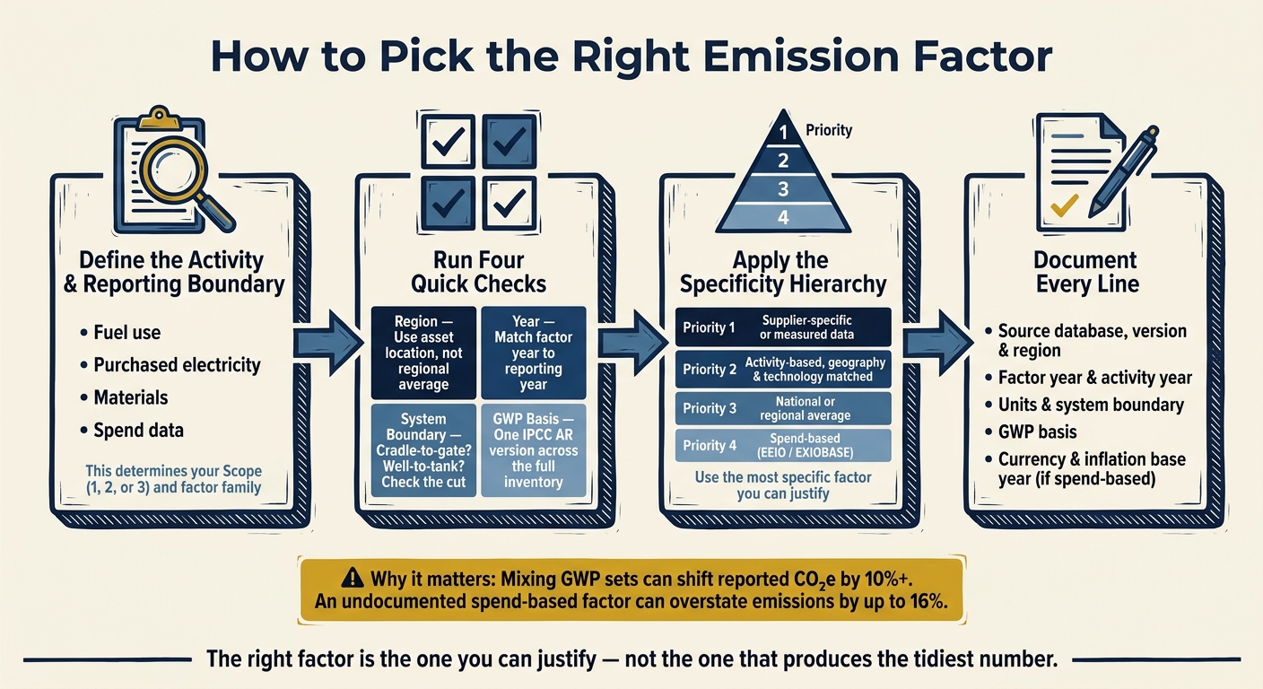
How to Pick the Right Emission Factor: A Step-by-Step Method
In due diligence, the factor you pick can change both the emissions footprint and the investment read-through. The method below gives you a clear order of checks that stands up to review. Use the same sequence for every line item.
Start with the activity and reporting boundary
Before you open any database, define the activity with care. Is it fuel use, purchased electricity, a material bought from a supplier, or spend data? That one call tells you which scope applies and which factor family to check first.
The reporting boundary matters just as much. A combustion factor covers direct emissions only. If your reporting boundary includes upstream fuel emissions, add those separately.
Check region, year, system boundary and GWP set
Once you know the activity and scope, run four quick checks before you accept any factor.
Region comes first. Grid factors can differ a lot by country, so use the asset’s location, not a broad regional average.
Year comes next. Match the factor year to the reporting year. Don’t use older versions unless you have a clear reason [4].
System boundary follows. Check the lifecycle cut: cradle-to-gate, cradle-to-grave, well-to-tank or tank-to-wheel. Use only the part your reporting needs.
GWP basis comes last. Use one IPCC GWP set across the inventory. Don’t mix assessment report versions [5].
Apply a hierarchy of specificity
When more than one factor seems to fit, use the table below to choose.
| Priority | Factor Type | When to Use |
|---|---|---|
| 1 | Supplier-specific or measured data | Verified product carbon footprint or utility-specific mix |
| 2 | Activity-based, geography and technology matched | Physical units; country and process known |
| 3 | National or regional average | No supplier or process detail |
| 4 | Spend-based (EEIO / EXIOBASE) | Only financial records available |
This hierarchy helps you defend the choice. Put simply: the right factor is the one you can justify, not the one that produces the tidiest number. If a reviewer asks why you used a national average instead of a supplier figure, your answer should be plain: supplier data was not available, and that choice was logged as an assumption. If one factor changes the total in a material way, swap the proxy for primary data [4].
If you have to fall back on spend-based factors, state the boundary and the reason in clear terms. Mixing methods without explanation makes the result harder to defend.
For each line item, record the source, year, boundary and GWP basis. Without that, the factor choice won’t hold up. Once you’ve picked the factor, document the source and assumptions line by line.
Why documentation must travel with every line
A factor is only defensible if each line carries its source and assumptions.
The minimum metadata to record per line
For each line item, record the source database, version, and region; factor year; activity year where that differs; units; system boundary; and GWP basis. If you used a spend-based factor, record the currency too, along with the base year used for any inflation adjustment.
Keep this information with the calculation itself, not tucked away in a separate note. That way, a reviewer can test the line without jumping between files. That record is what makes the line auditable, comparable, and defensible.
How factor choice changes investment conclusions
This matters because factor choice can change the answer in a very direct way. Different databases or vintages can push a line across materiality thresholds or make progress look better than it is [6].
Mixing different GWP bases within one inventory can shift reported CO₂e by 10% or more [5]. An undocumented spend-based factor without inflation adjustment can overstate emissions by up to 16% [6]. These are not edge cases. They’re the sort of quiet errors that tend to show up during due diligence or audit, when the cost of fixing them is much higher. One choice of database, reference year, or currency base can move the reported total more than a year of operational reductions.
Conclusion: a clear factor policy beats a defensible estimate
All of this points to one simple rule: write your factor policy before you start calculating.
Emission factors turn activity data into CO₂e. But the “right” factor isn’t one-size-fits-all. It depends on the activity type, geography, vintage, boundary, and whether the unit lines up properly.
Set the hierarchy before the analysis begins. Put primary or supplier-specific data first, matched activity factors next, and spend-based proxies last. If one factor has a material effect on the total, that’s your signal to go back and get better primary data.
For private markets teams, a written factor policy is what makes the work hold up in diligence and assurance settings. It should cover the factor hierarchy, the metadata you need, consistency rules, and a validation step. Factor selection is where credibility is earned.